Statistical analysis of two populations of Haworthia mirabilis (V.Poelln.) M.B.Bayer

M.B.Bayer & L.M.Loucka

Introduction:

In discussing H. rossouwii (Aloe 38:31, 2001), Bayer mentions the possible continuity with H. mirabilis var. sublineata.  But any comment like this is complicated by the problems of variation, description and circumscription.  We want to discuss the variation in the latter element and indicate further where the problems are in the delineating species and varieties.  It seems that one of the assumptions of classical plant taxonomy is that of linear dichotomy, black and white, this species or that, and also that there is hierarchical and consistent in-group similarity to some unstipulated degree.  Haworthia, and particularly the subgenus Haworthia, presents a problem to those interested in the genus in that the classification is confused and that identifications are difficult.  Attempts been made to explain that the classification is confused by the perceptions associated with classical taxonomy, and that the sharp and precise discontinuities suggested by a ‘key’ to the taxa, simply do not occur in the subgenus Haworthia, in fact they do not occur in many other genera, and this simple truth seems to be difficult for some to accept.

Thus this article includes a report of a study done on a batch of seedlings of H. mirabilis var. sublineata.  It shows that there is very little probability that one could quantify separation of this from other populations presumed to be the same species.

Outcomes in the biological world are influenced by genetics and environmental factors, but also by chance events. It is because of the probability of chance events that knowledge of statistics is essential to scientific research and our studies of the genus Haworthia.

Plants have parts that can be mechanically measured in terms of spread, height, width, length, thickness, arc; or counted as in the number of leaves or offsets.  Other attributes like colour, and surface texture are more subjective.  When we observe leaf structures in Haworthia our perception often tries to make sense and draw patterns from many subtle characteristics viz. this plant is species X because it has a pattern that matches our experience.  But our brains can be easily fooled when we try to compartmentalize.  When we subject our observations to measurement we begin to sort out the characteristics we use to describe one plant, population, or species from another.  Viewing this collection in the leisure of the greenhouse, we can see that some leaves were thicker or longer than others, but are they “really”?  That is, are they significantly thicker, or longer?  When we count the number of leaves, or measure their length can we make some statements to compare and differentiate one population from another?  Do the differences we measure translate into differences in overall size and shape of the leaf?  Let’s investigate this further by formulating the following question:

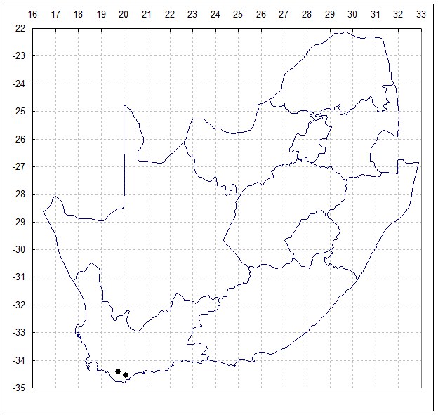
Method: Seed of H. mirabilis var. sublineata was field collected at the type locality south of Bredasdorp in April 1997, accessioned as MBB6639.  By Sept.2000 these seedlings were at flowering size and 71 plants were available for the study.  A second study sample was taken from a population of H. mirabilis var. triebneriana from Fairfield, west of Napier (MBB6643).  H. mirabilis is very widespread and this Napier population is apparently no more or less variable than many others known.

Population 1, MBB6639 – 3420CA South of Bredasdorp.  April 1997.  North facing steep rocky slope, Table Mountain Sandstone with grassy mountain fynbos.

Population 2, MBB6643 – 3419DD Fairfield 15km West of Napier.  April 1997.  North facing shale ridge, Bokkeveld Shale with grassy renosterveld.

Prior to this study, an attempt was made to reduce the size of the group of MBB6639 seedlings by discarding any single clones which were obviously similar.  To do this Bayer tried to arrange the plants according to similarity. He could not find any pattern, and each plant appeared to be fairly unique.  Five plants were removed in order to propagate them vegetatively, and for this study a further four clones were removed which were either obviously atypical or retarded.  Four smaller apparently under grown clones were retained in the final study batch of 62.

A first attempt was again made to try and identify groups by visual comparison.  This proved impossible to do.  Attempting to reduce the size of the set by the identification of “identical” pairs also failed.  No two plants were sufficiently similar to be regarded as near to identical.  The simplest way forward was then to match the plants as closely as possible into pairs, repeating the process five times.  After pairing, the pairs were broken and the plants returned to a random array.  Pairing was then done again by picking up any one clone and finding the best match.  Some re-sorting was done in order to accommodate the last of the clones as the pairing process neared an end.  In some cases clones which could not be adequately paired were compared over all the others to find the best match.  Although an attempt was made to score the “goodness” of pairs, this proved difficult to do and an inconsistent result was obtained.  Some clones simply proved more difficult than others to match.

With five attempts, the total pairings was 310.  Sixteen clones were unpaired.  Of the pairings, 210 were unique, in 74 cases the same two clones were paired, in 18 cases the same clones were paired three times, in 8 cases four times and in two cases, all 5 times.  This shows that there is very little consistent pattern in the group as a whole when trying to match or differentiate based simply on assessing visual cues.

Recognising now that no progress was being made, Bayer considered what ‘characters’ he was using in his visual assessment and then quantified his observations.  Some of the characters used in the visual process could include:

a. Size
b. Colour
c. Leaf number
d. Leaf width
e. Leaf length
f. Leaf thickness
g. Leaf recurvature: i. compactness, ii.  erect or reflexed
h. Leaf marginal spination
i. Leaf upper surface: i. translucence, ii.  texture, iii. venation, iv.  basal opacity, v. basal marking
j. Leaf lower surface (as above)
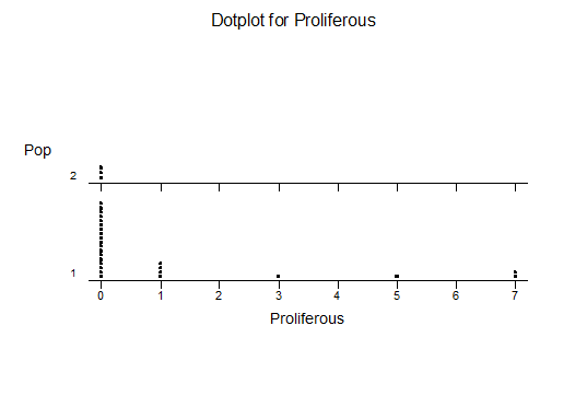
k. Proliferation (off-setting)

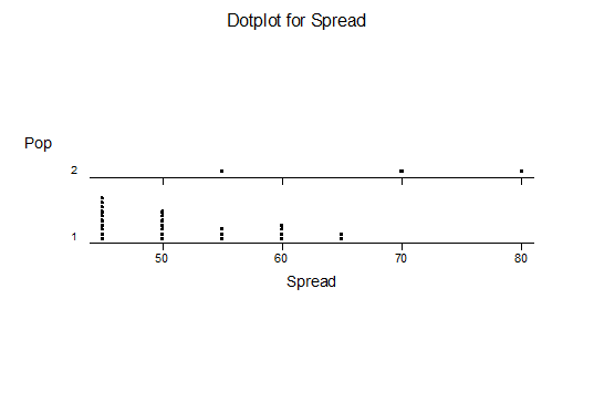
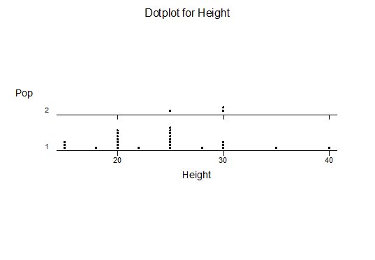
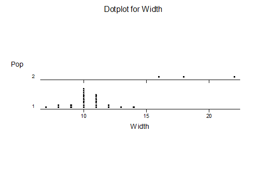
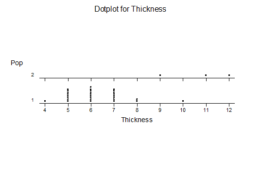
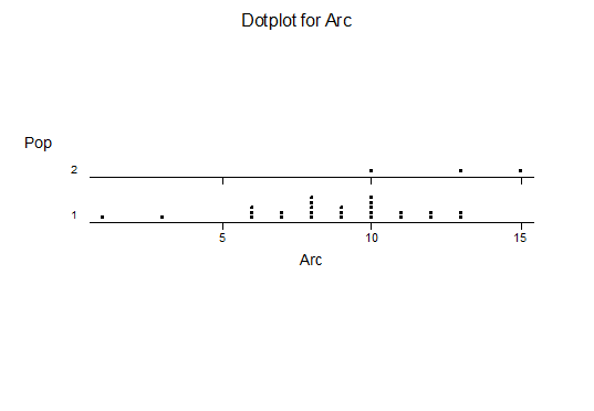
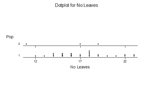
For statistical analysis it was decided to use the measured spread of the leaves from the tips of the most extended leaves, the height reached by the highest leaf tip measured from the base, the width, length, and thickness of the largest leaf at maximum, and to measure the arching of such leaves by the gap between a line drawn from base to tip and the lower leaf surface (i.e. recuravture).  A subjective measurement was made of leaf surface roughness, size and number of spines, and degree of tubercles. The resulting data was analyzed by a Dotplot for each characteristic and a Two-sample T-test used to assess the null hypothesis.

Descriptive Statistics

The MBB6639 plants show the classic bell-shaped normal distribution for most characteristics with the exception of spread and proliferation (off set count).  Perhaps the population culling of the runts and natural survival account for the truncated spread data.  In time more of the clones may have offsets and thus show a different distribution.  For the other characteristics we can see a central tendency and data points spread to the left and right.  It’s this central tendency, or average (statistically called the mean) that we’ll study further.

Hypothesis Testing

Question: Are plants from the two populations in this study of the same or different sizes and shape?

Hypotheses: The difference in the average physical characteristics between the two populations is zero; i.e. the null hypothesis (Ho:).  If the difference between the means of the samples is among those that would occur rarely by chance when the null hypothesis is true, then the null hypothesis is rejected and the investigator describes the results as statistically significant.  That is, the difference between the average of each population characteristic must be great enough to conclude if the populations are the same or different.

Prediction: If the leaves of the two populations are the same size, then the spread, height, width, length, thickness, and arc of the populations should be the same.

Analysis:

The P value we subject our data to is 0.05, or a 5% chance that we would accept that the difference is the means of the two populations is zero when in fact it isn’t.

A null hypothesis is not accepted just because it is not rejected.  Data that is not sufficient to show convincingly that a difference between means is not zero do not prove that the difference is zero. Such data may even suggest that the null hypothesis is false but not be strong enough to make a convincing case that the null hypothesis is false.  For example, if the probability value P were 0.15, then one would not be ready to present one’s case that the null hypothesis is false to the (properly) skeptical scientific community.  More convincing data would be needed to do that. However, there would be no basis to conclude that the null hypothesis is true.  It may or may not be true, there just is not strong enough evidence to reject it.

What can we conclude?  The two populations appear to be different for leaf width and thickness.  For all other characteristics we just don’t have enough data to make any conclusive statement.

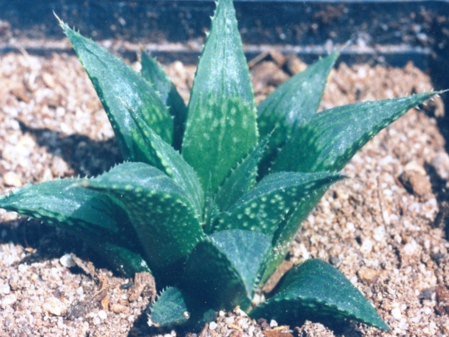
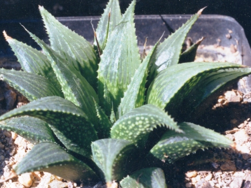
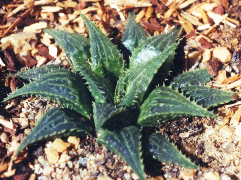
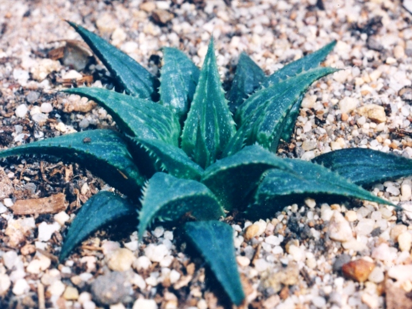
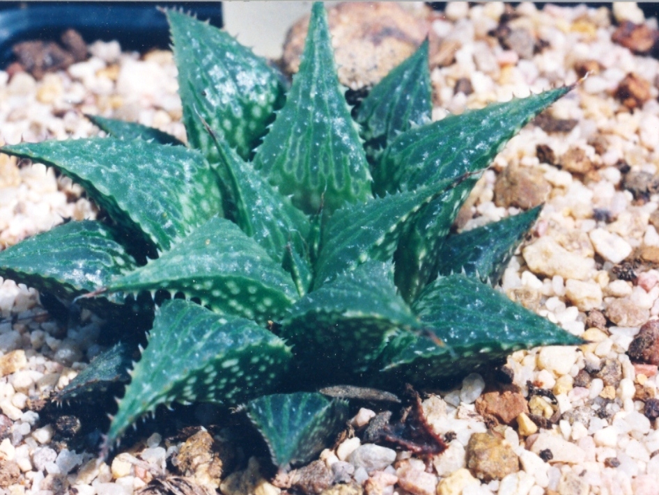
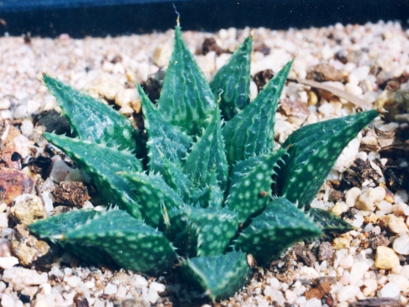
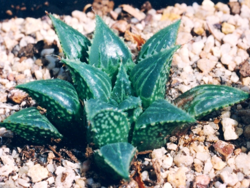
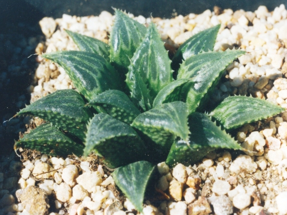
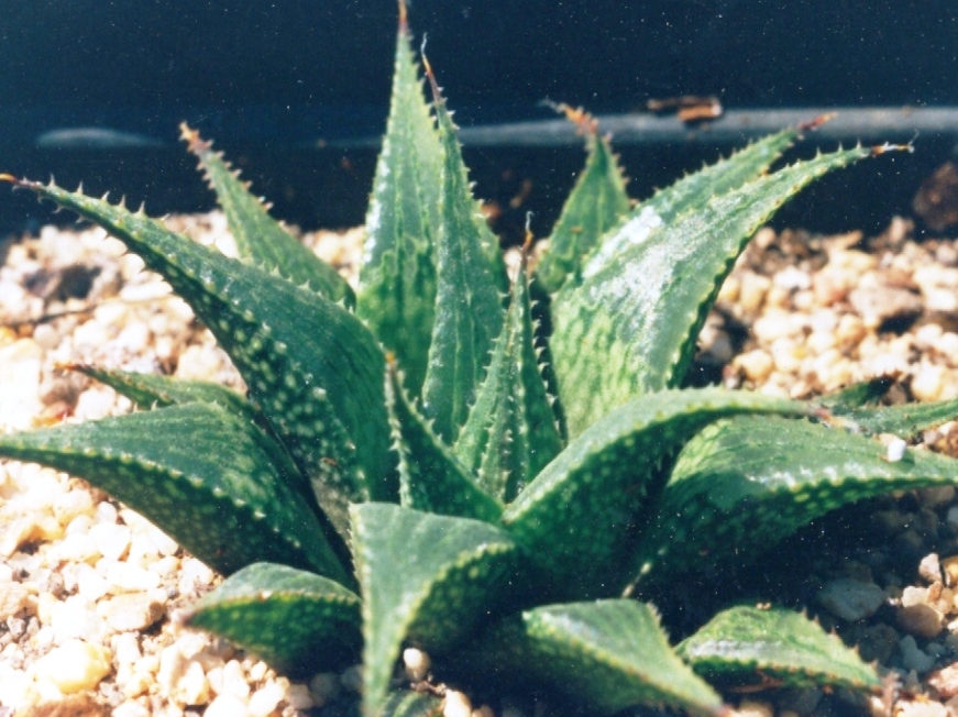
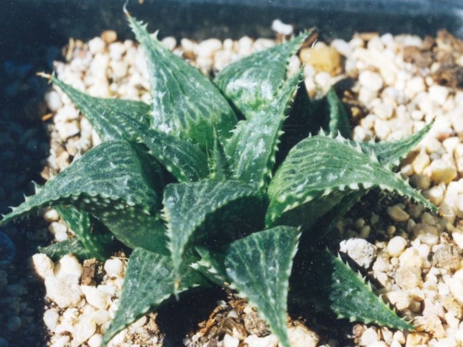
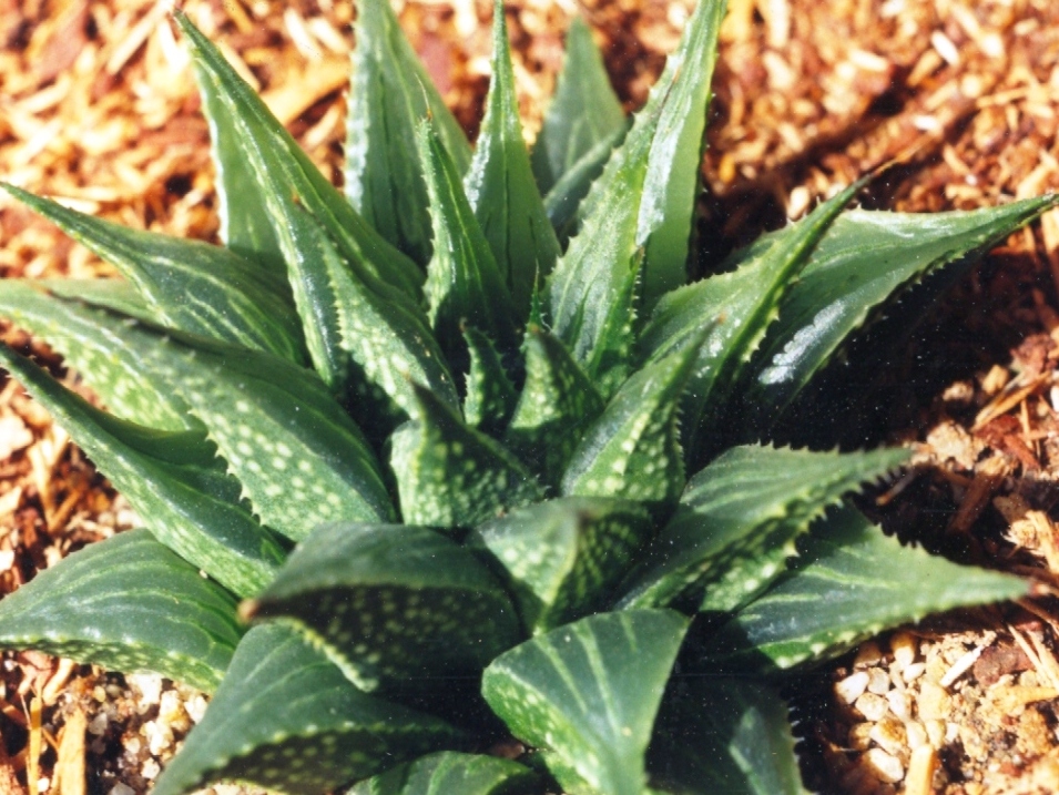
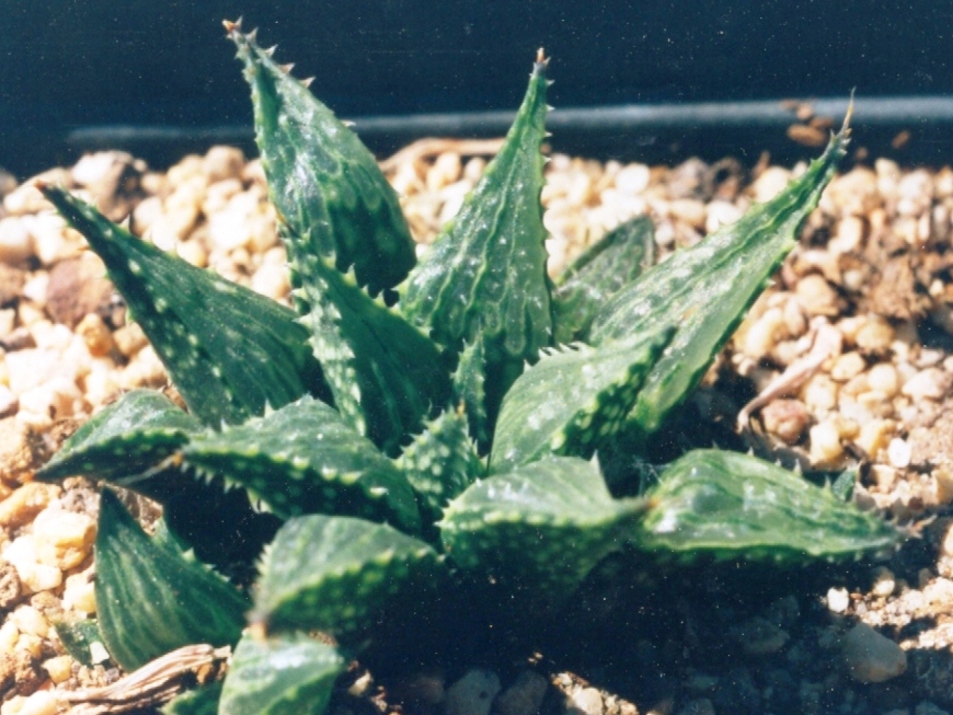
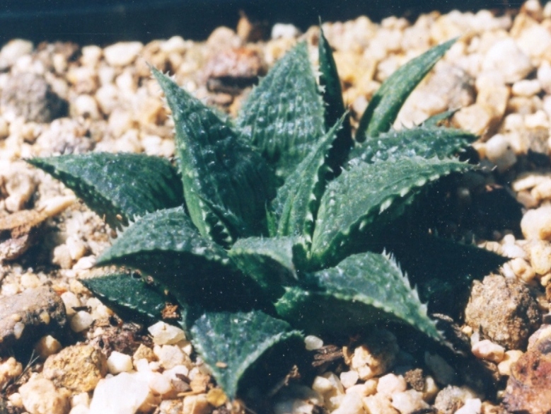
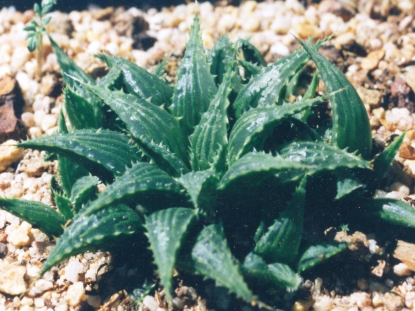
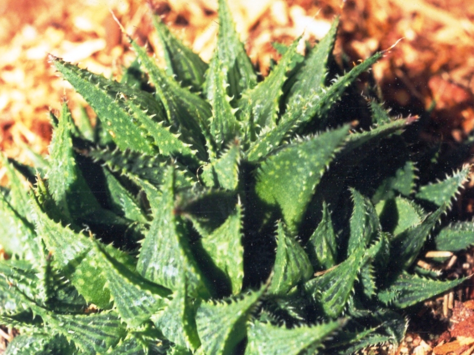
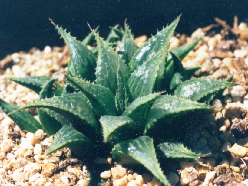
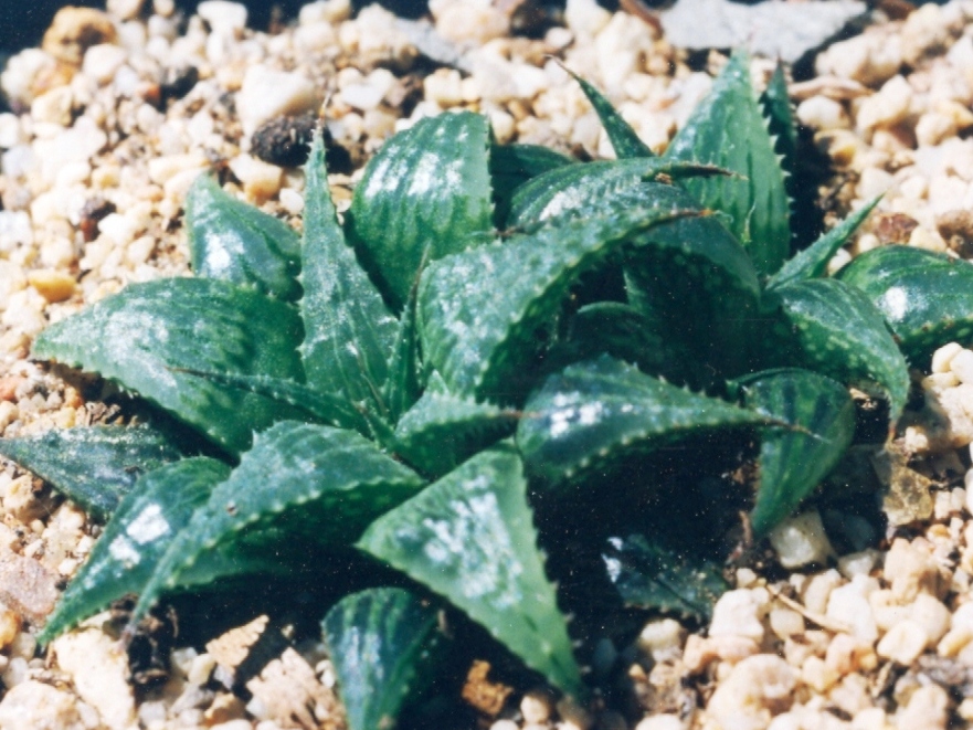
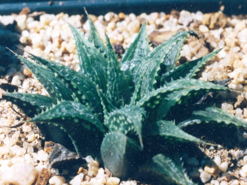
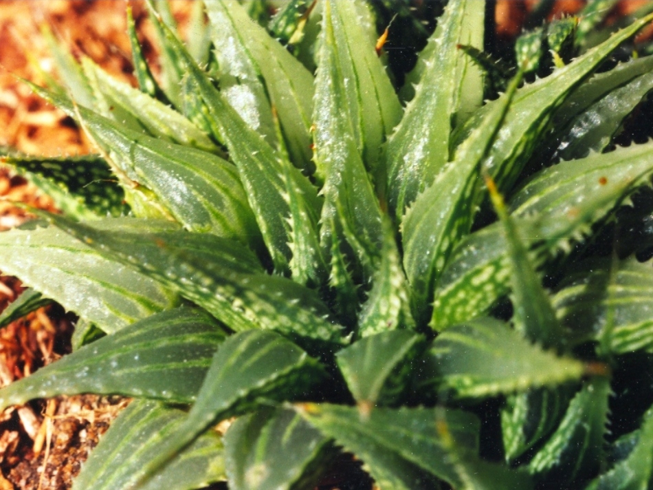
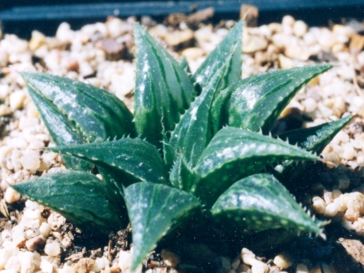
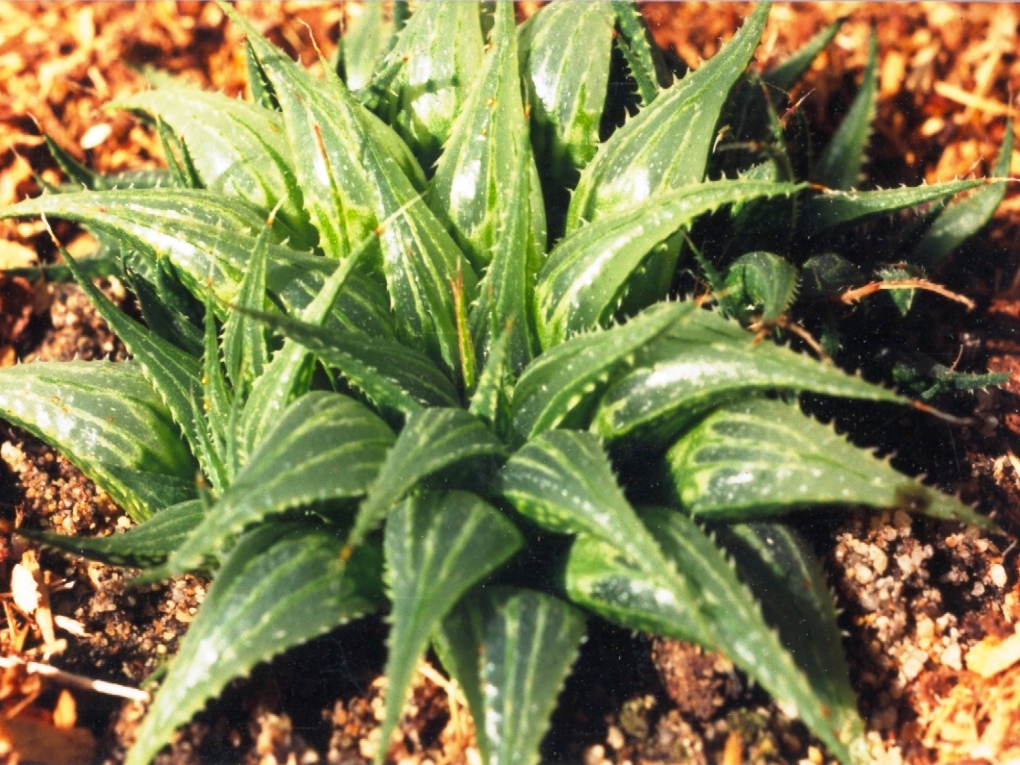
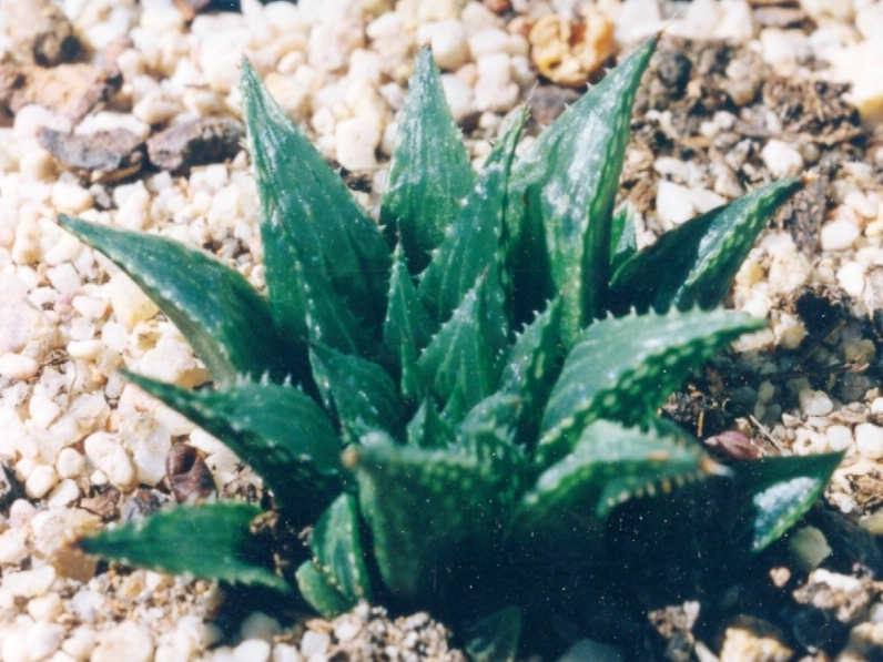
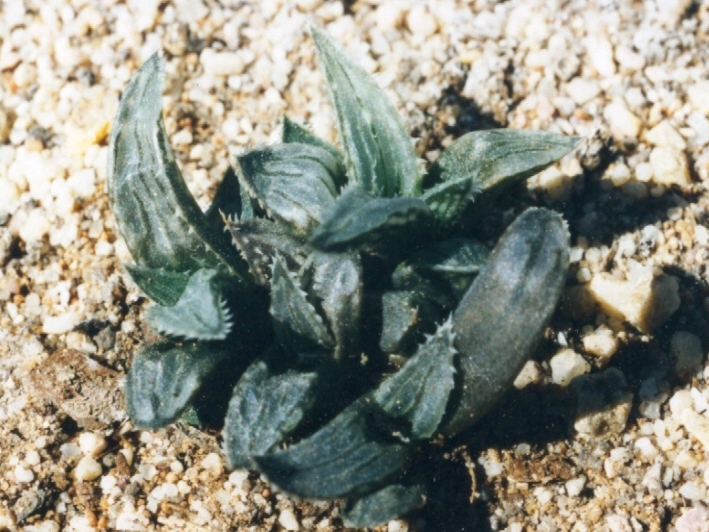
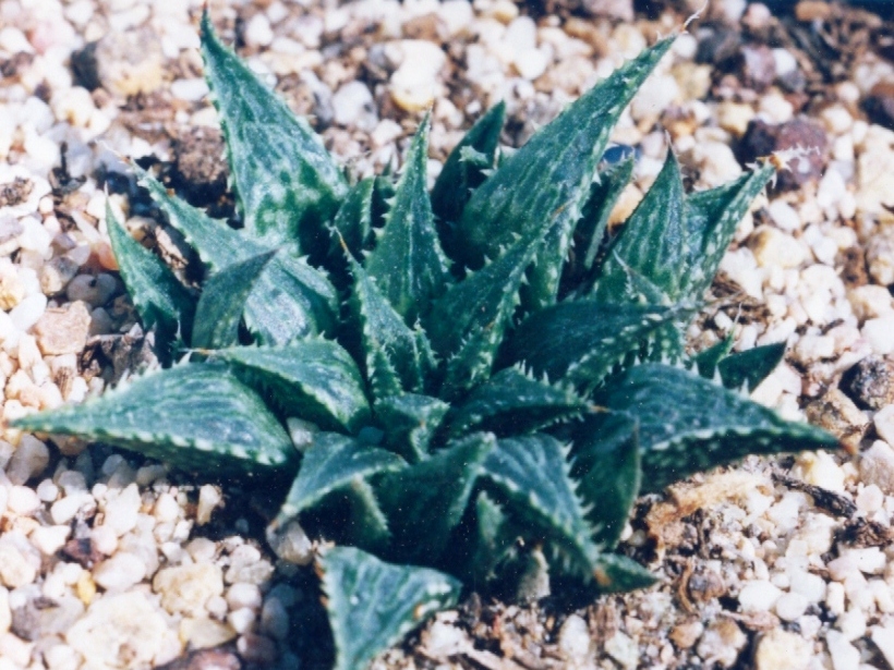
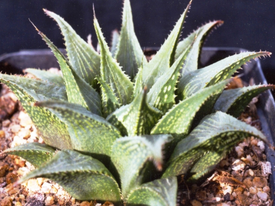
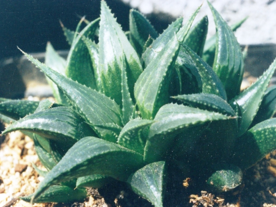
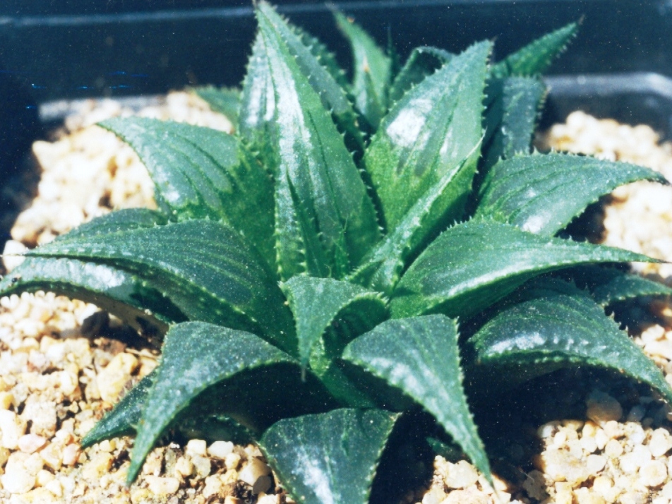
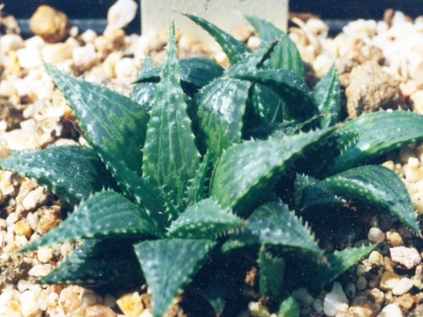
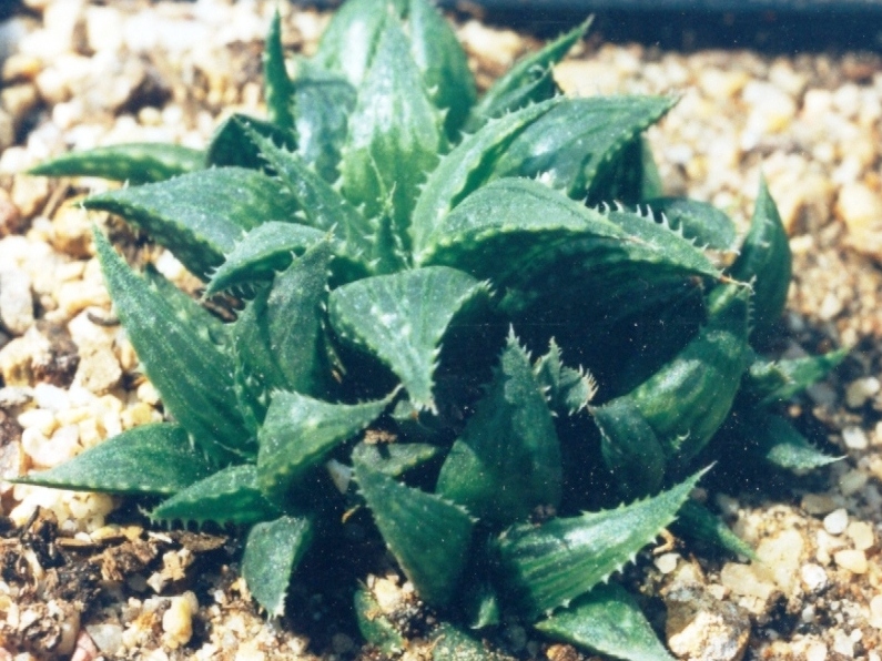
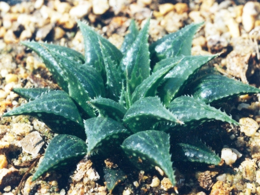
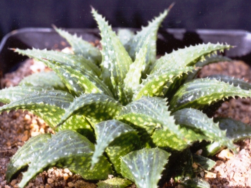
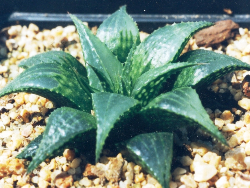
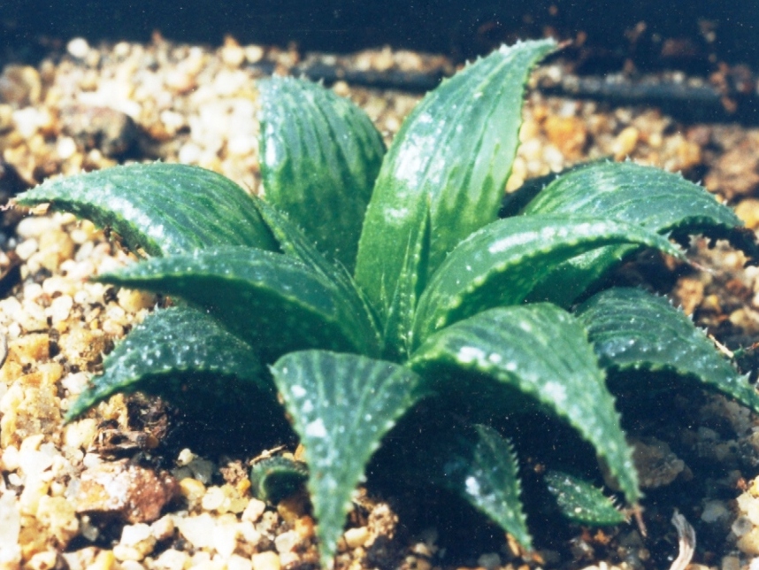
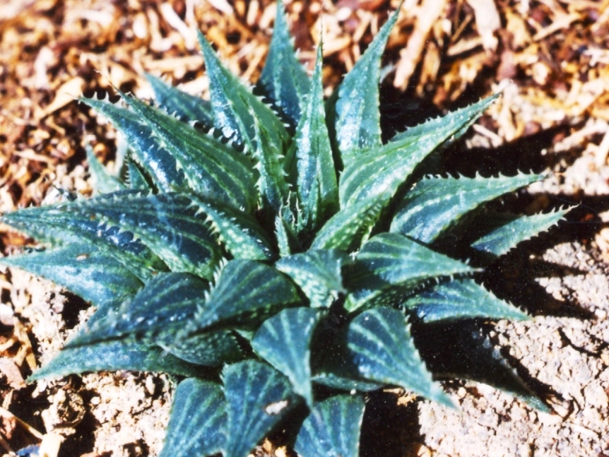
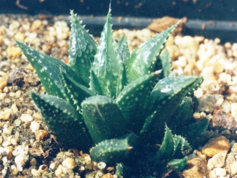
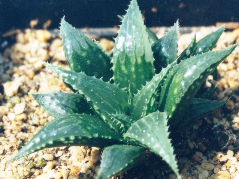
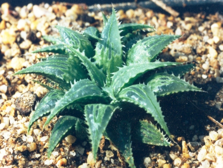
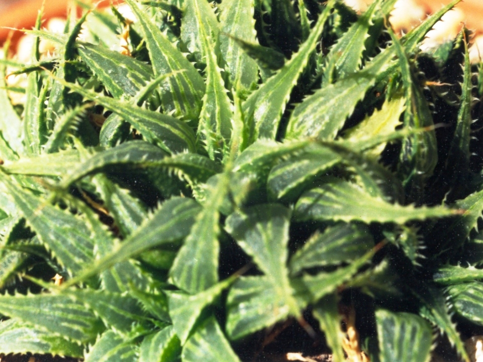
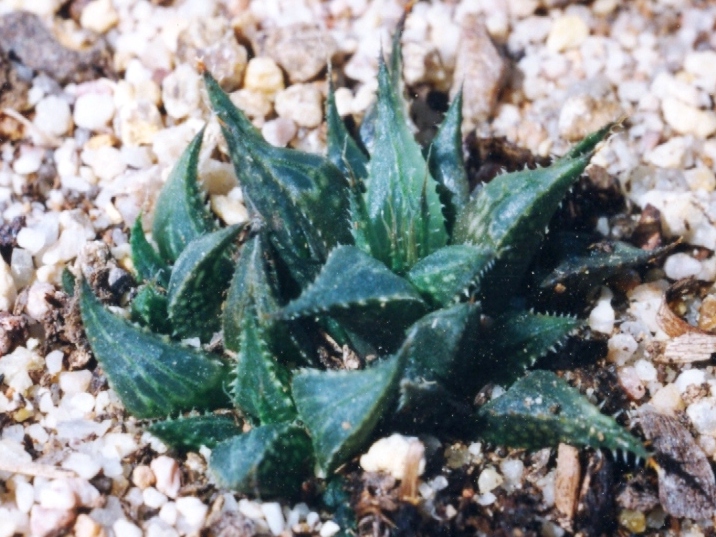
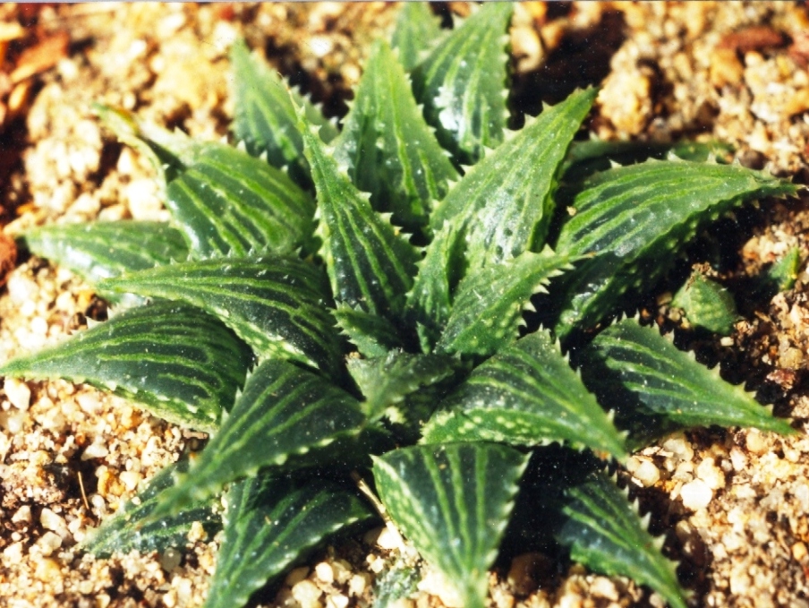
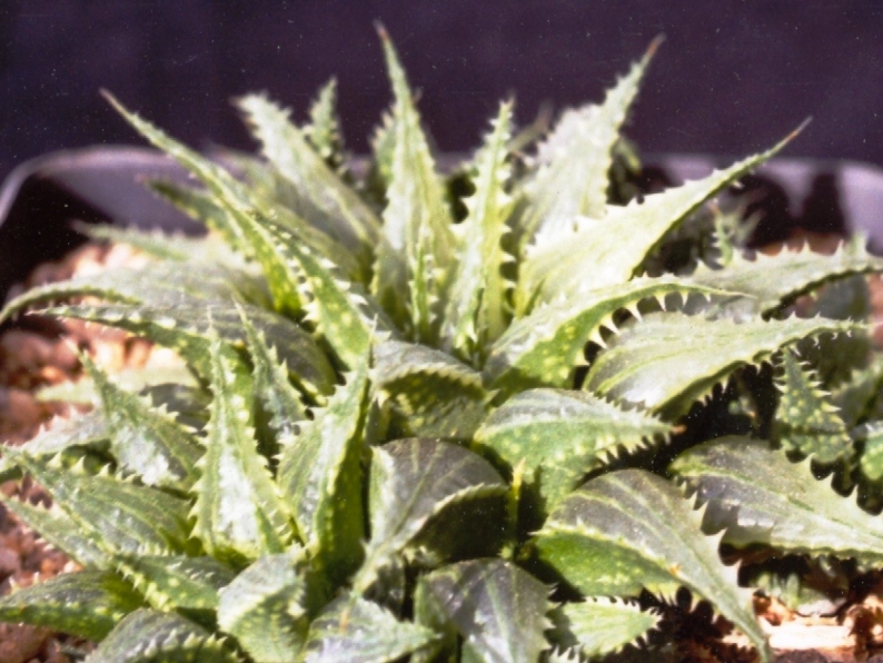
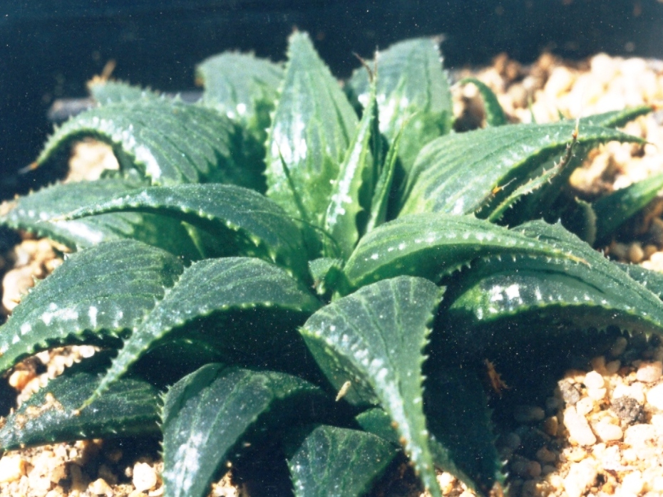
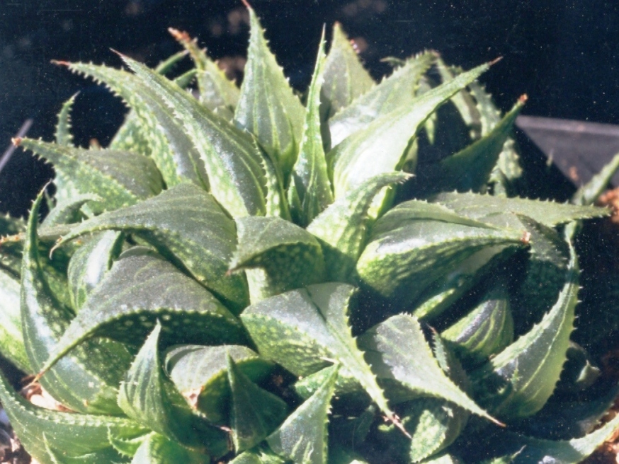
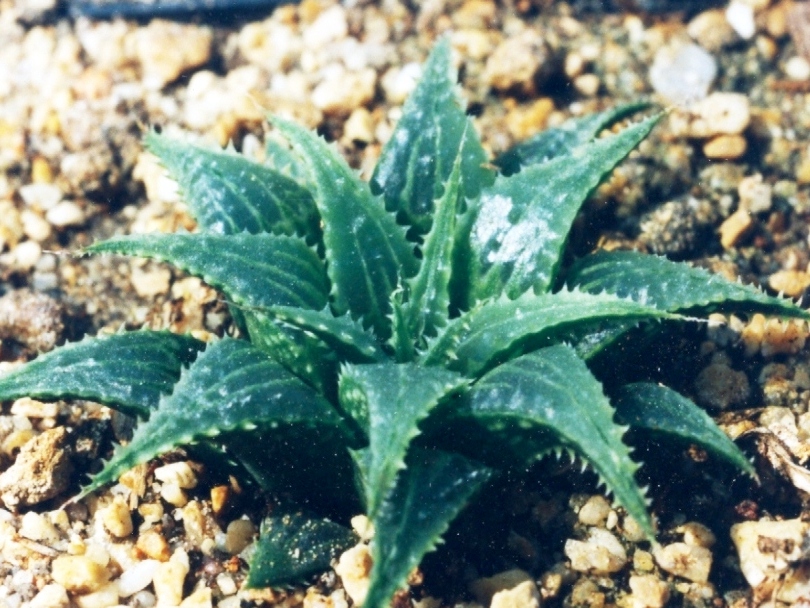
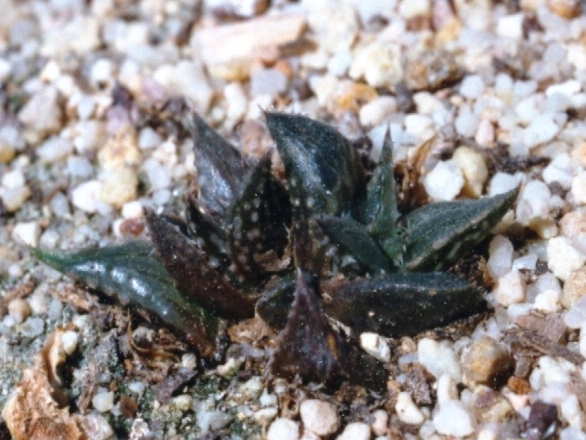
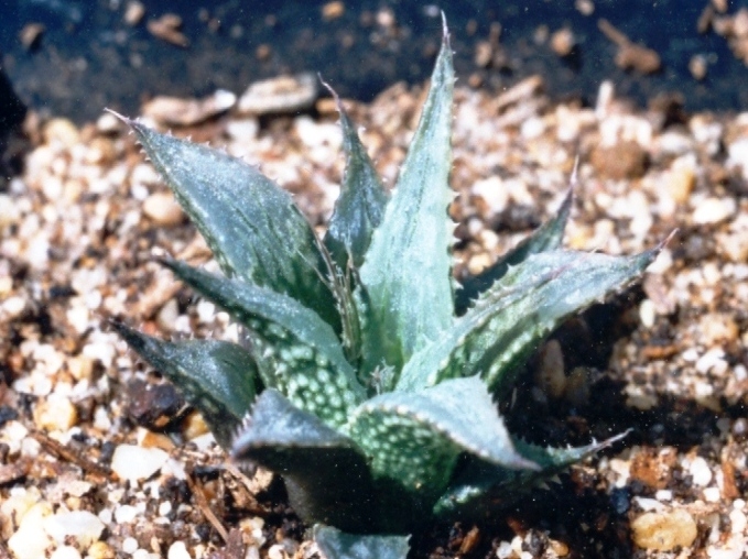
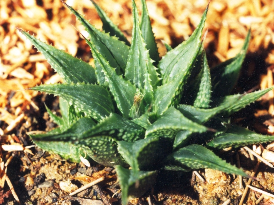
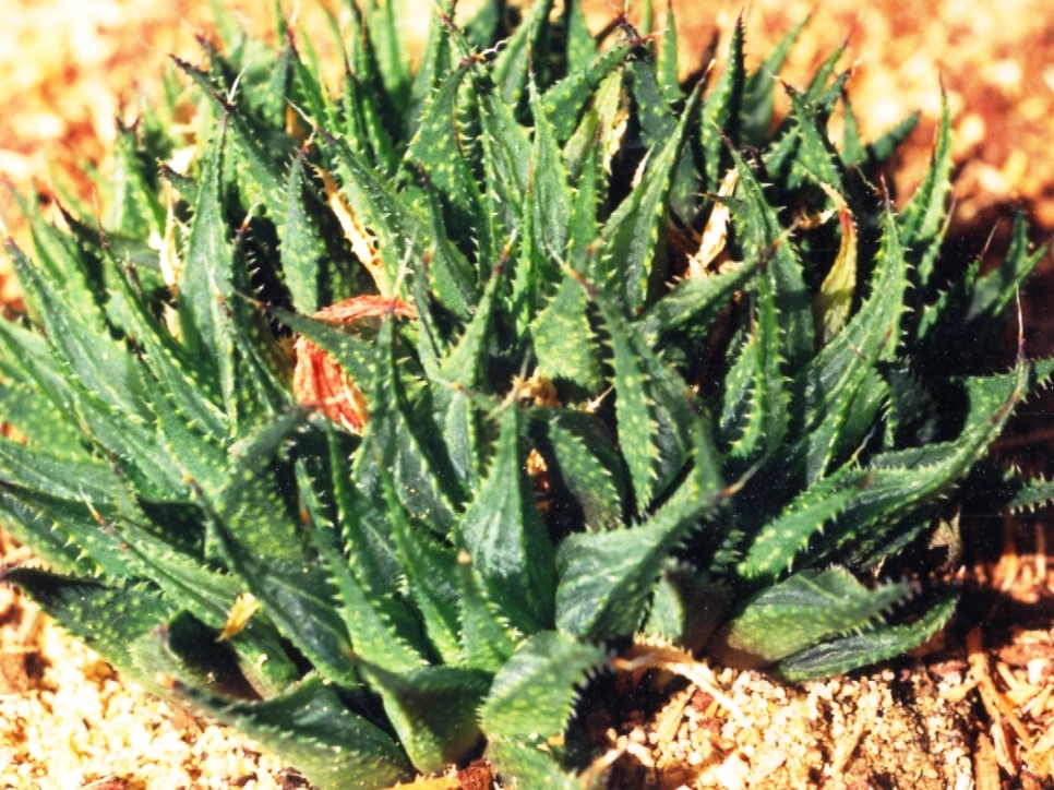
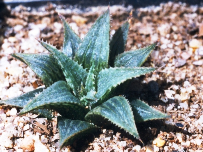
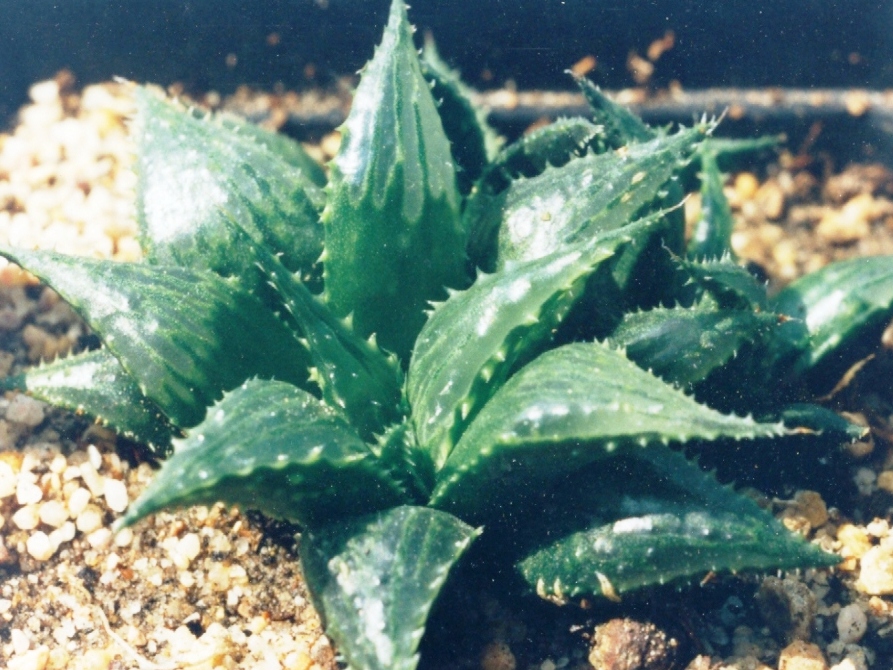
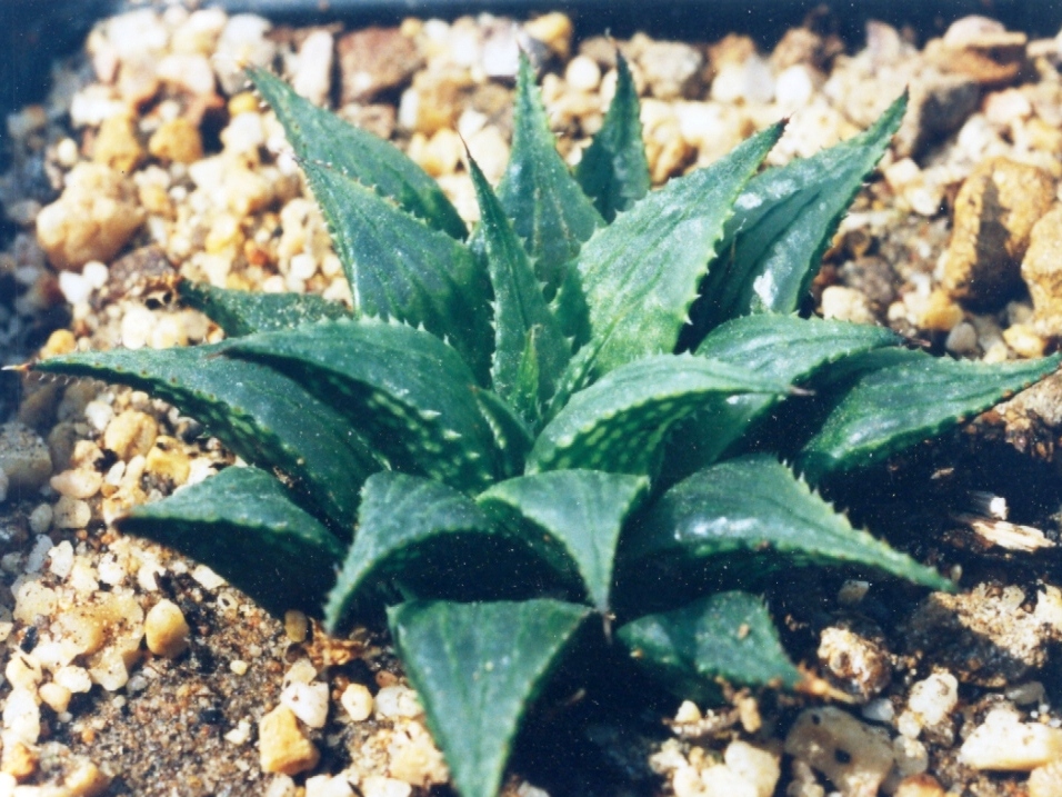
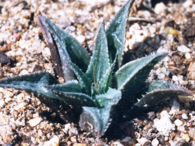
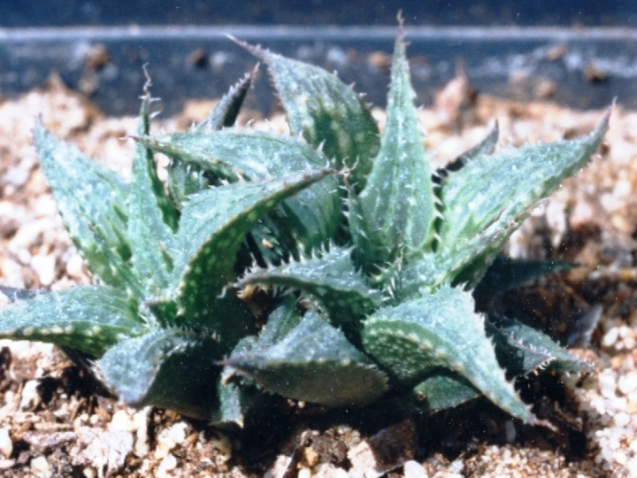
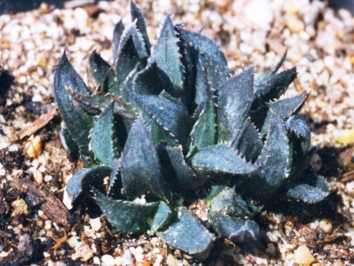
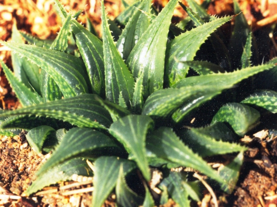
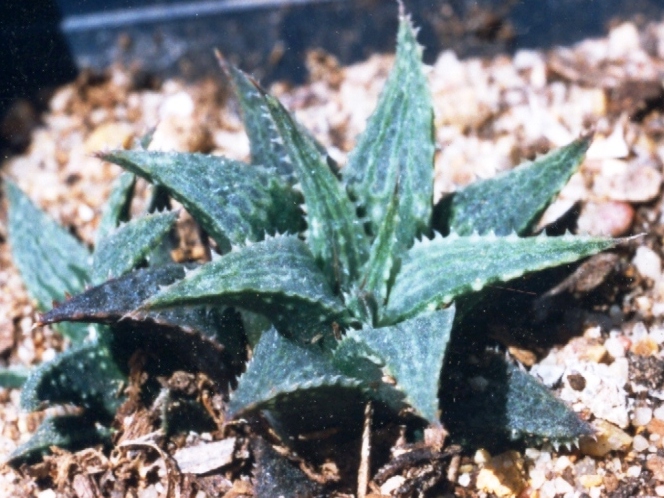
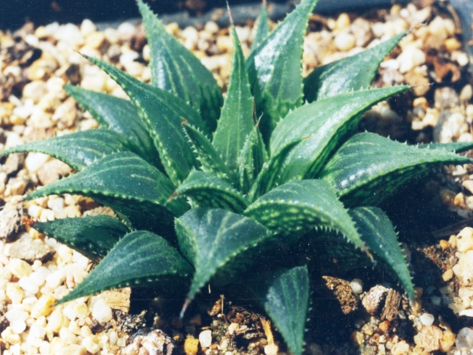
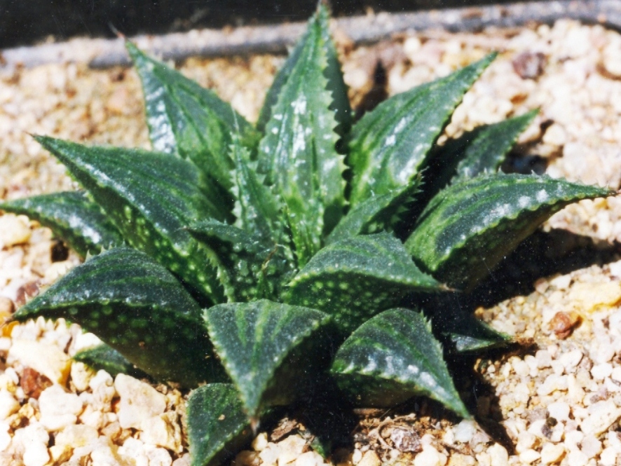
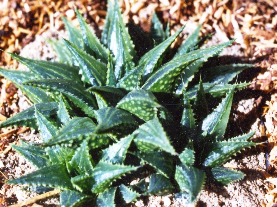
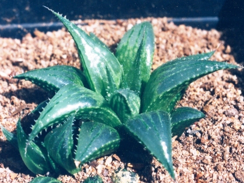
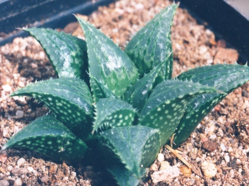
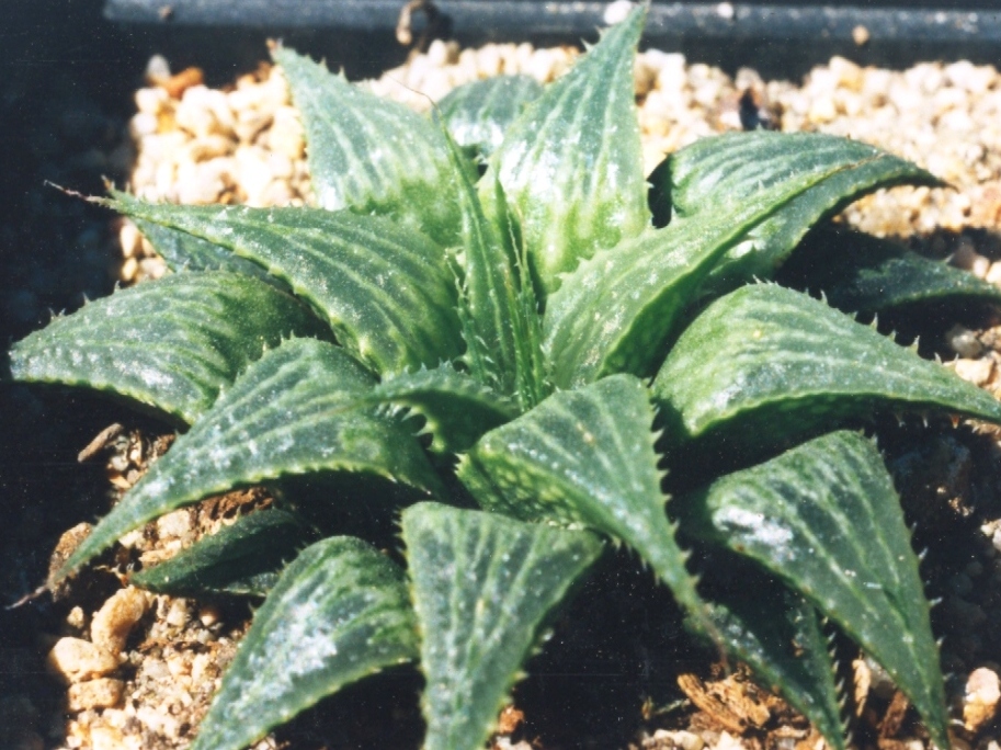
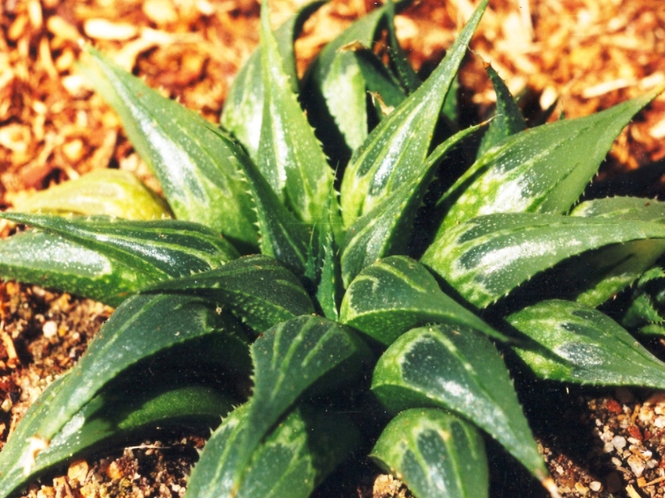
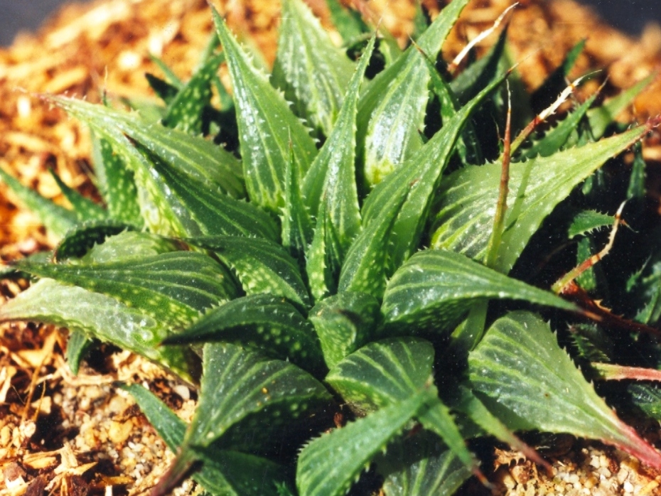
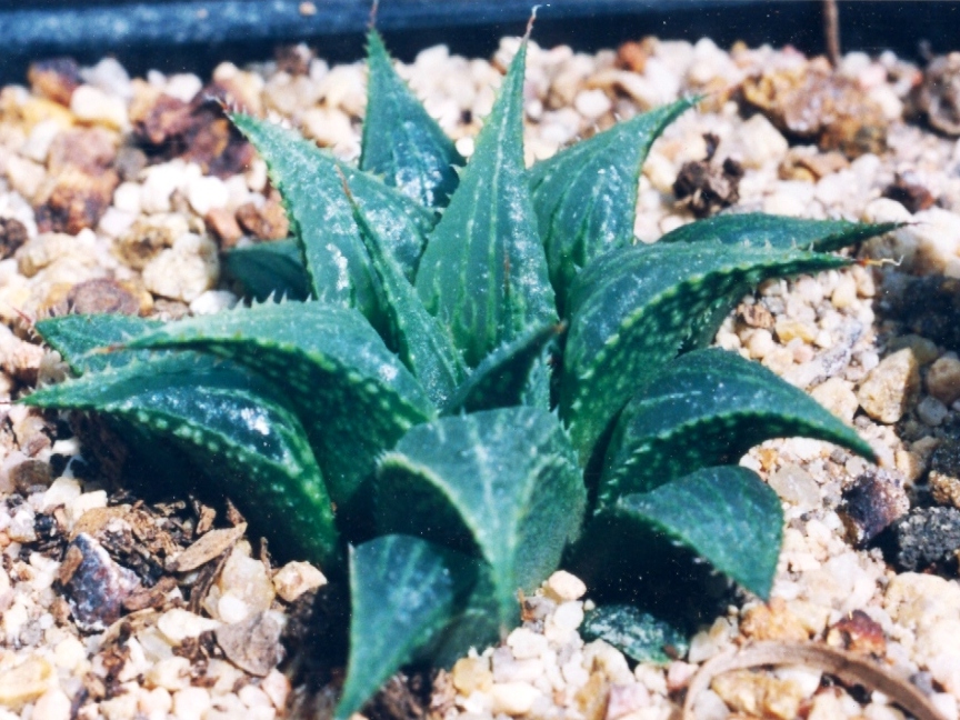
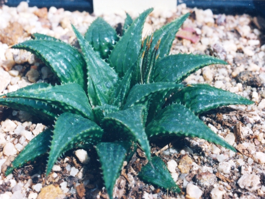
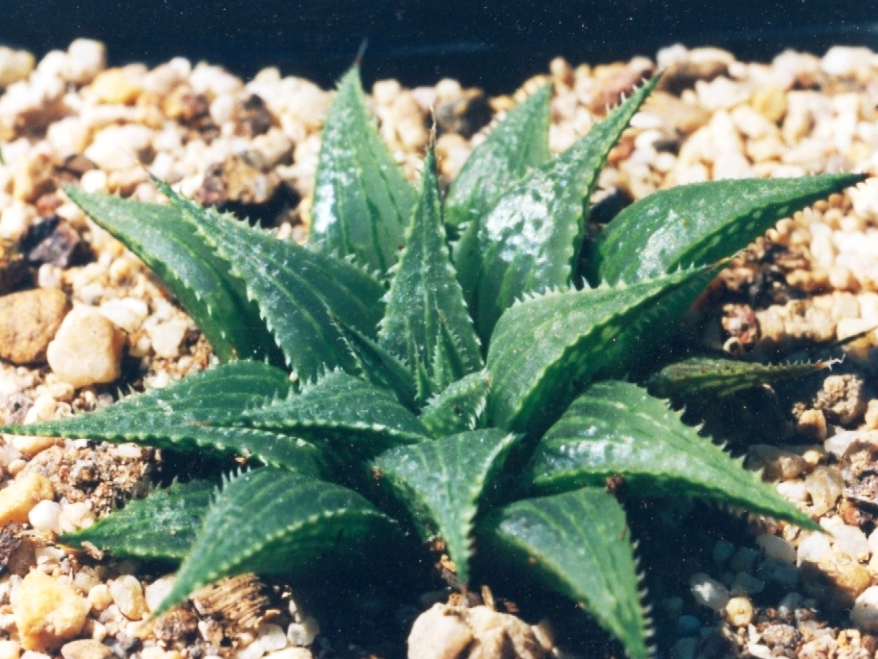
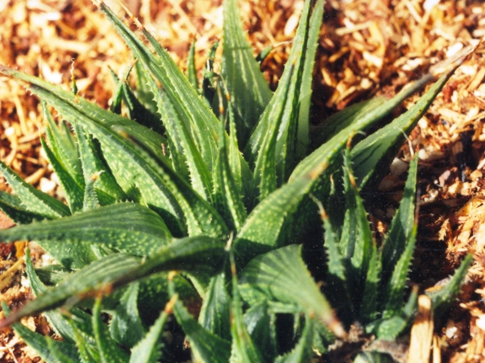
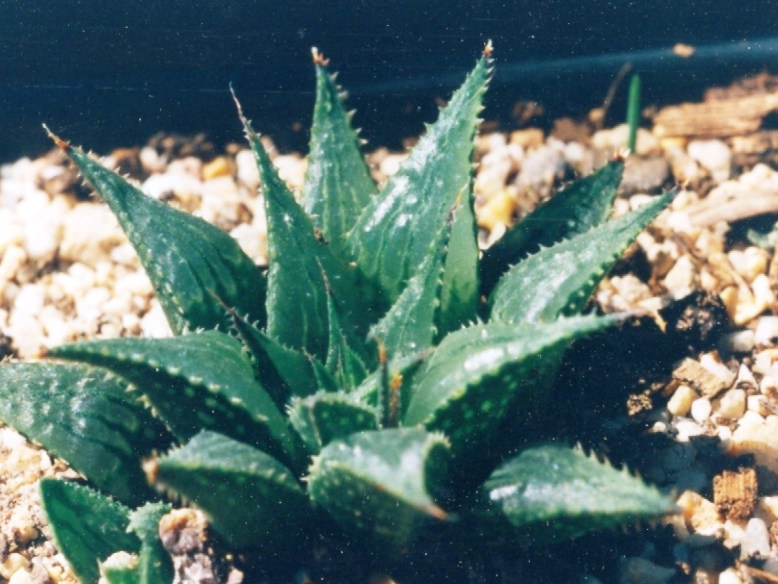
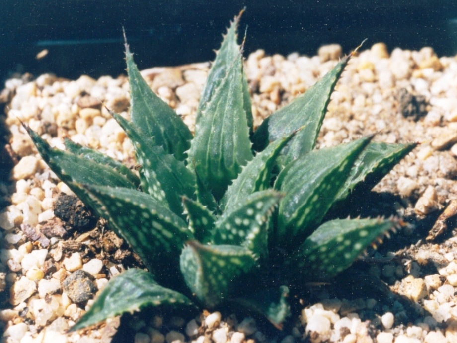
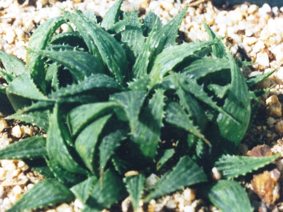
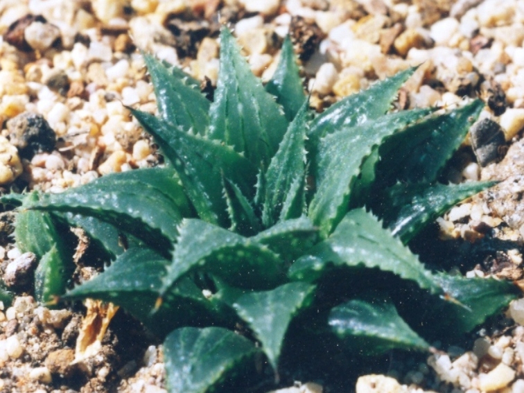
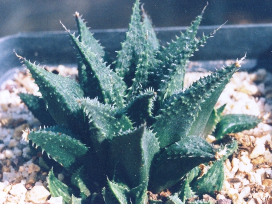
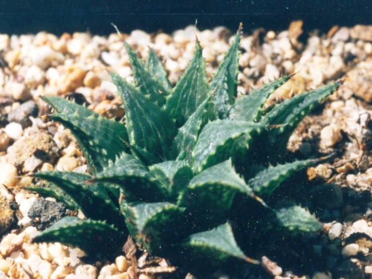
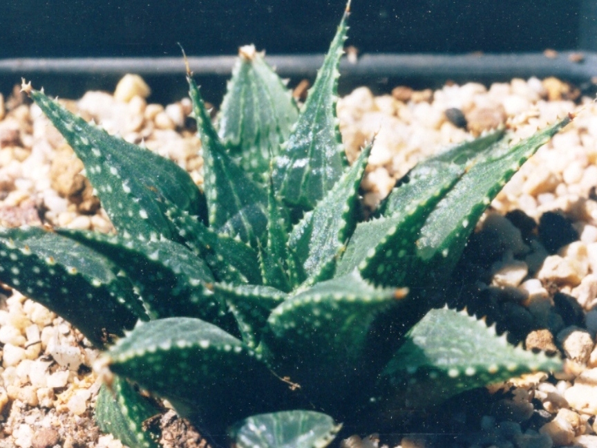
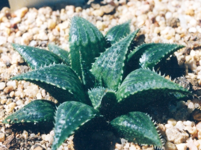
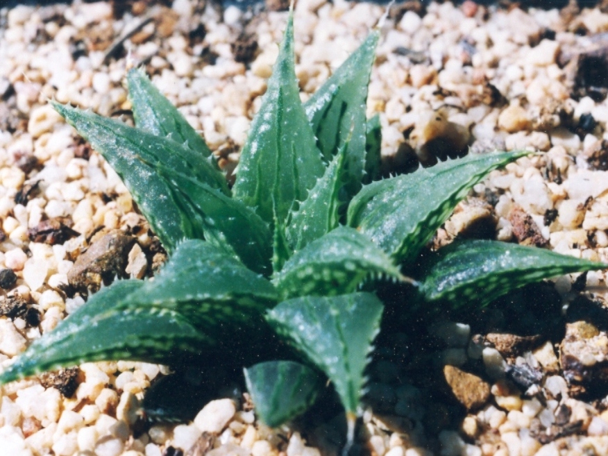
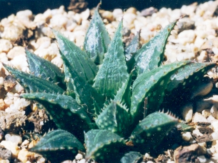
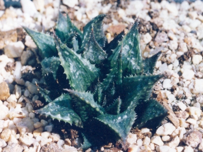
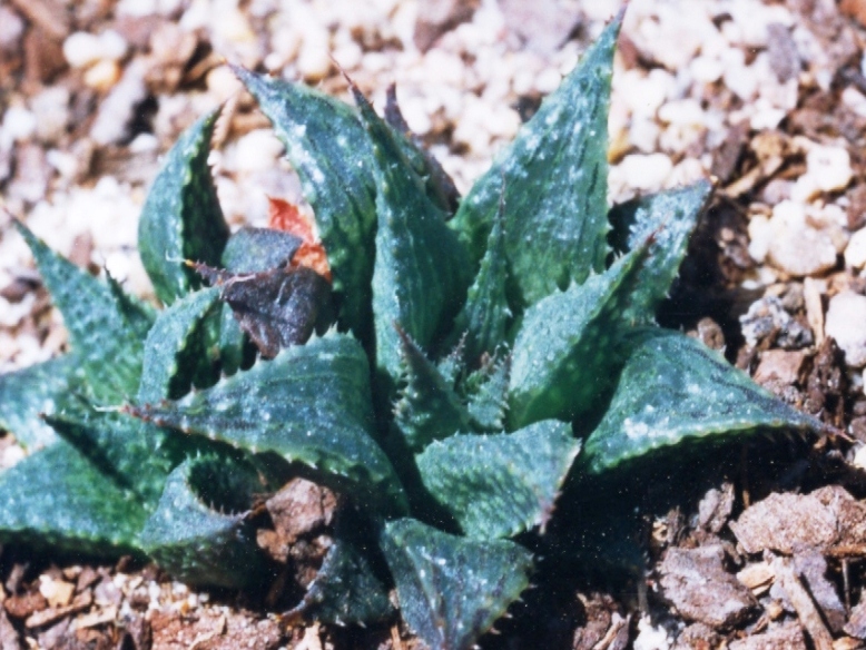
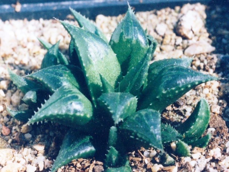
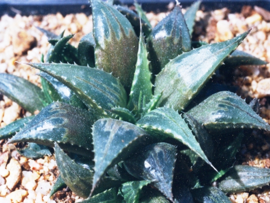
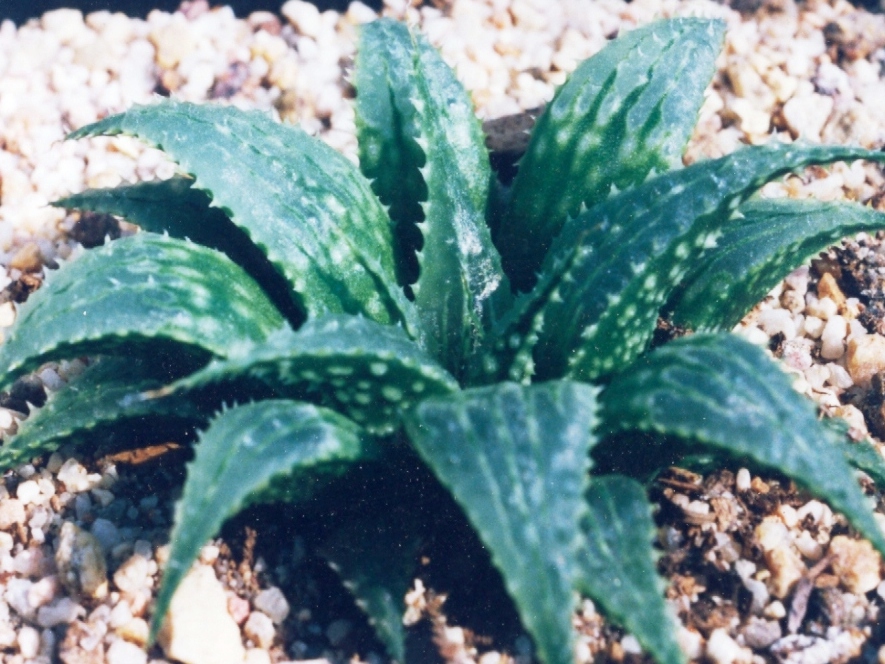
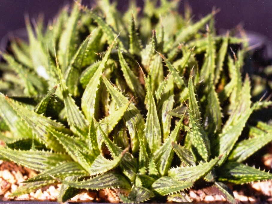
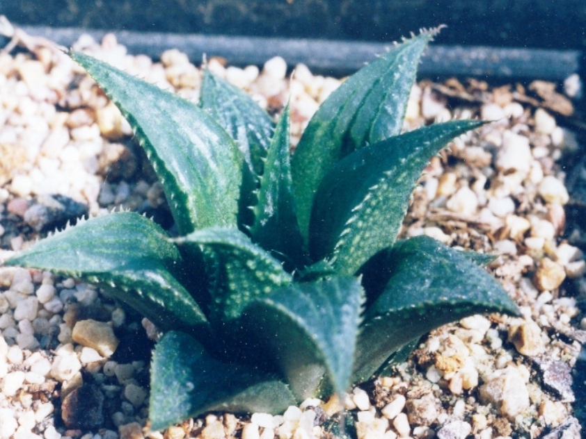
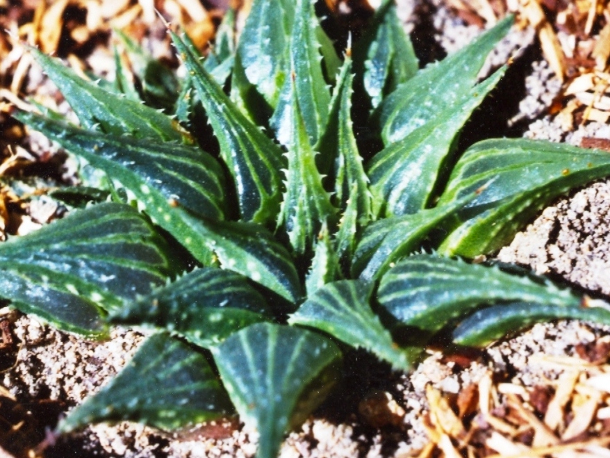
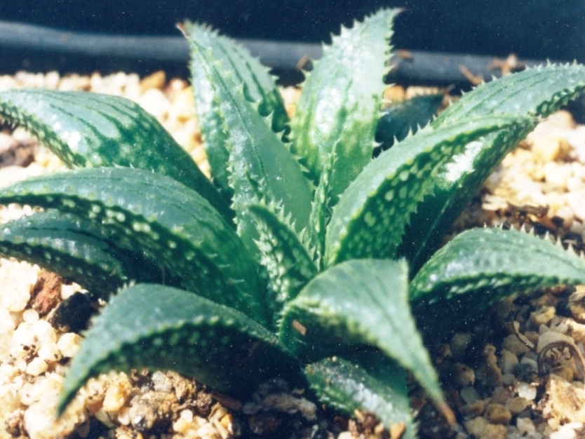
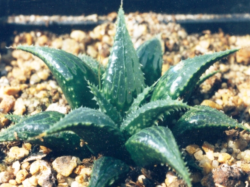
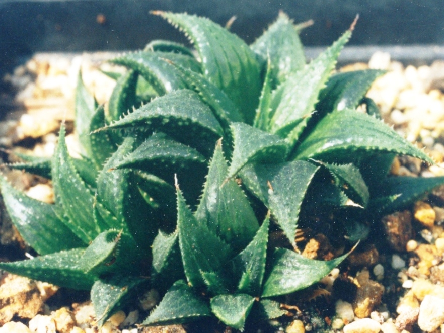
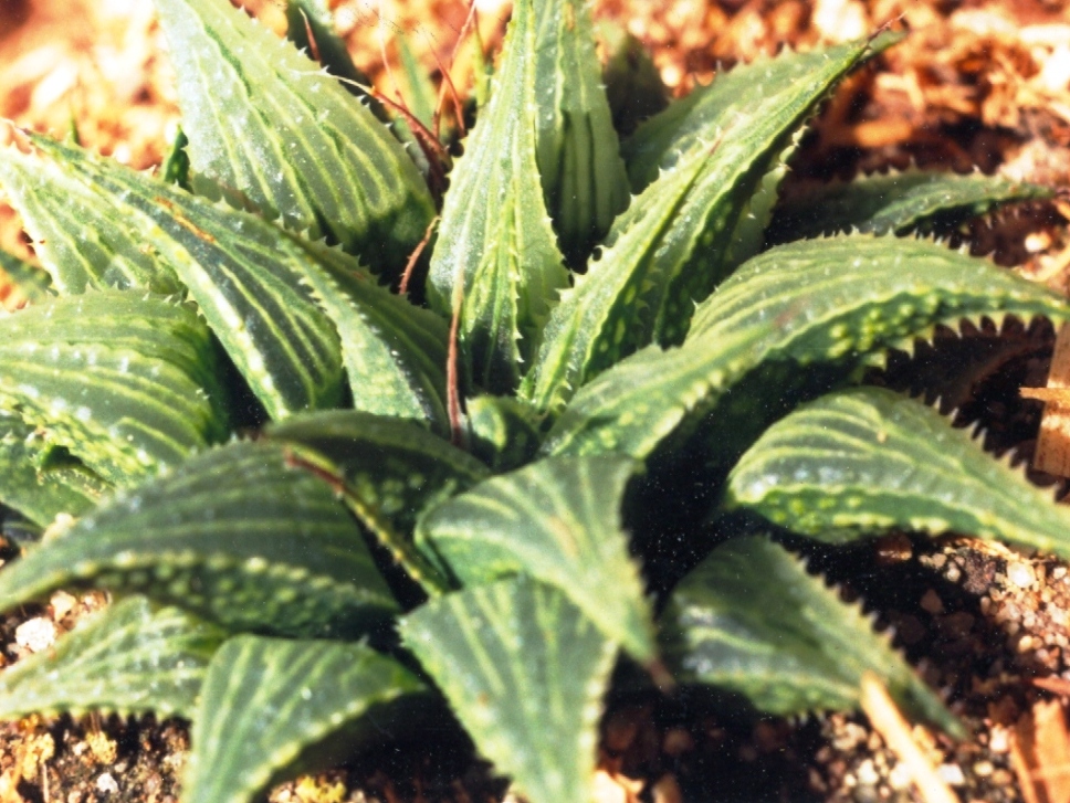
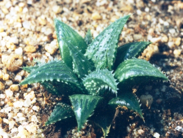
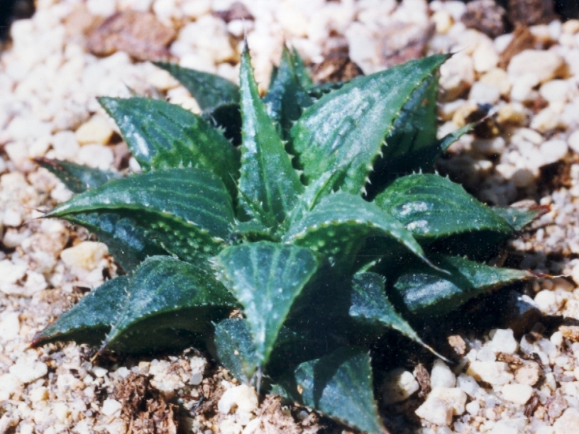
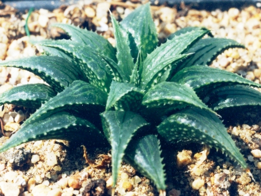
We have illustrated the individual clones for the reader to appreciate how different the individual plants may be, and also to consider that the appearances of the plants will vary according to growing medium, exposure to light, season and watering.

Discussion and Conclusion:

Our observation is that a statistical approach simply does not penetrate the nuance of difference that visual observation can discern.  The data we present is valuable only in that it illustrates the variation within the population MBB6639.  The coefficients of variation of the characters used are so high that larger samples would be required to provide more reliable statistics.  In this study we have used a second population 6643 which is obviously different. At Bredasdorp there are in fact two other populations. One of these is on a north-facing river bank in among river-eroded sandstone boulders, while across the river about 250M away is a smaller population in Bokkeveld shale.  Plants from all three populations are relatively easy to identify.  The riverine boulder plants have fewer stumpier and more reflexed leaves, while the shale plants have erect leaves.  To what extent these differences are “real” cannot be proven without a replication of the seed collecting and propagating effort done for 6639.  In the context of ALL the populations which may comprise the species H. mirabilis it is quite evident that this is impractical.

• 

• 

• 

• 

• 

• 

• 

• 

• 

• 

• 

• 

• 

• 

• 

• 

• 

• 

• 

• 

• 

• 

• 

• 

• 

• 

• 

• 

• 

• 

• 

• 

• 

• 

• 

• 

• 

• 

• 

• 

• 

• 

• 

• 

• 

• 

• 

• 

• 

• 

• 

• 

• 

• 

• 

• 

• 

• 

• 

• 

• 

• 

• 

• 

• 

• 

• 

• 

• 

• 

• 

• 

• 

• 

• 

• 

• 

• 

• 

• 

• 

• 

• 

• 

• 

• 

• 

• 

• 

• 

• 

• 

• 

• 

• 

• 

• 

• 

• 

• 

• 

• 

• 

• 

• 

• 

• 

• 

• 

• 

• 

• 

• 

• 

• 

• 

• 

• 

• 

• 

• 

• 

• 

• 

• 

• 

• 

• 

• 

• 

• 

• 

• 

• 

• 

• 

• 

• 

• 

• 

• 

• 

• 

• 

• 

• 

• 

• 

• 

• 

• 

• 

• 

• 

• 

• 

• 

• 

• 

• 

• 

• 

• 

• 

• 

• 

• 

• 

• 

• 

• 

• 

• 

• 

• 

• 

• 

• 

• 

• 

• 

• 

• 

• 

• 

• 

• 

•